You can evaluate model deployments in a deployment space to gain insights about your model performance. When you configure evaluations, you can analyze evaluation results and model transaction records directly in your spaces.
- Required services
- watsonx.governance
- watsonx.ai
Your basic workflow includes these tasks:
- Open a project. Projects are where you can collaborate with others to work with data.
- Build and save a machine learning model. There are various tools to build a model, such as, an AutoAI experiment, a Jupyter notebook, an SPSS Modeler flow, or a Pipelines. See Analyzing data and working with models.
- Deploy and test your model in a deployment space.
- Configure evaluations in the deployment space.
- Evaluate your model performance.
Read about how to evaluate deployments in spaces
watsonx.governance evaluates your model deployments to help you measure performance and understand your model predictions. When you configure model evaluations, watsonx.governance generates metrics for each evaluation that provide different insights that you can review. watsonx.governance also logs the transactions that are processed during evaluations to help you understand how your model predictions are determined.
Read more about evaluating deployments in spaces
Learn about other ways to evaluate models in Watson OpenScale
Watch a video about how to evaluate deployments in spaces
 Watch this video to preview the steps in this tutorial. There might be slight differences in the user interface shown in the video. The
video is intended to be a companion to the written tutorial.
Try a tutorial to evaluate deployments in spaces
In this tutorial, you will complete these tasks:
- Task 1: Create a project based on a sample
- Task 2: Deploy the model
- Task 3: Configure evaluations in a deployment space
- Task 4: Evaluate the model
- Task 5: Observe the model monitors for quality
- Task 6: Observe the model monitors for fairness
- Task 7: Observe the model monitors for drift
- Task 8: Observe the model monitors for explainability
Tips for completing this tutorial
Here are some tips for successfully completing this tutorial.
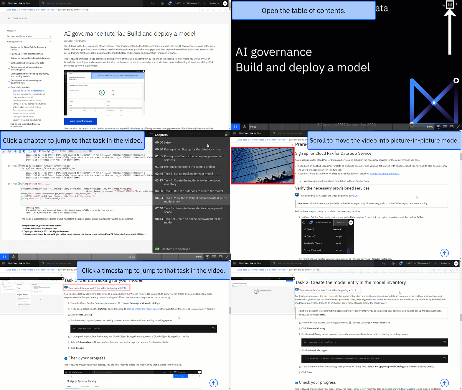
Use the video picture-in-picture
The following animated image shows how to use the video picture-in-picture and table of contents features:
Get help in the community
If you need help with this tutorial, you can ask a question or find an answer in the Cloud Pak for Data Community discussion forum.
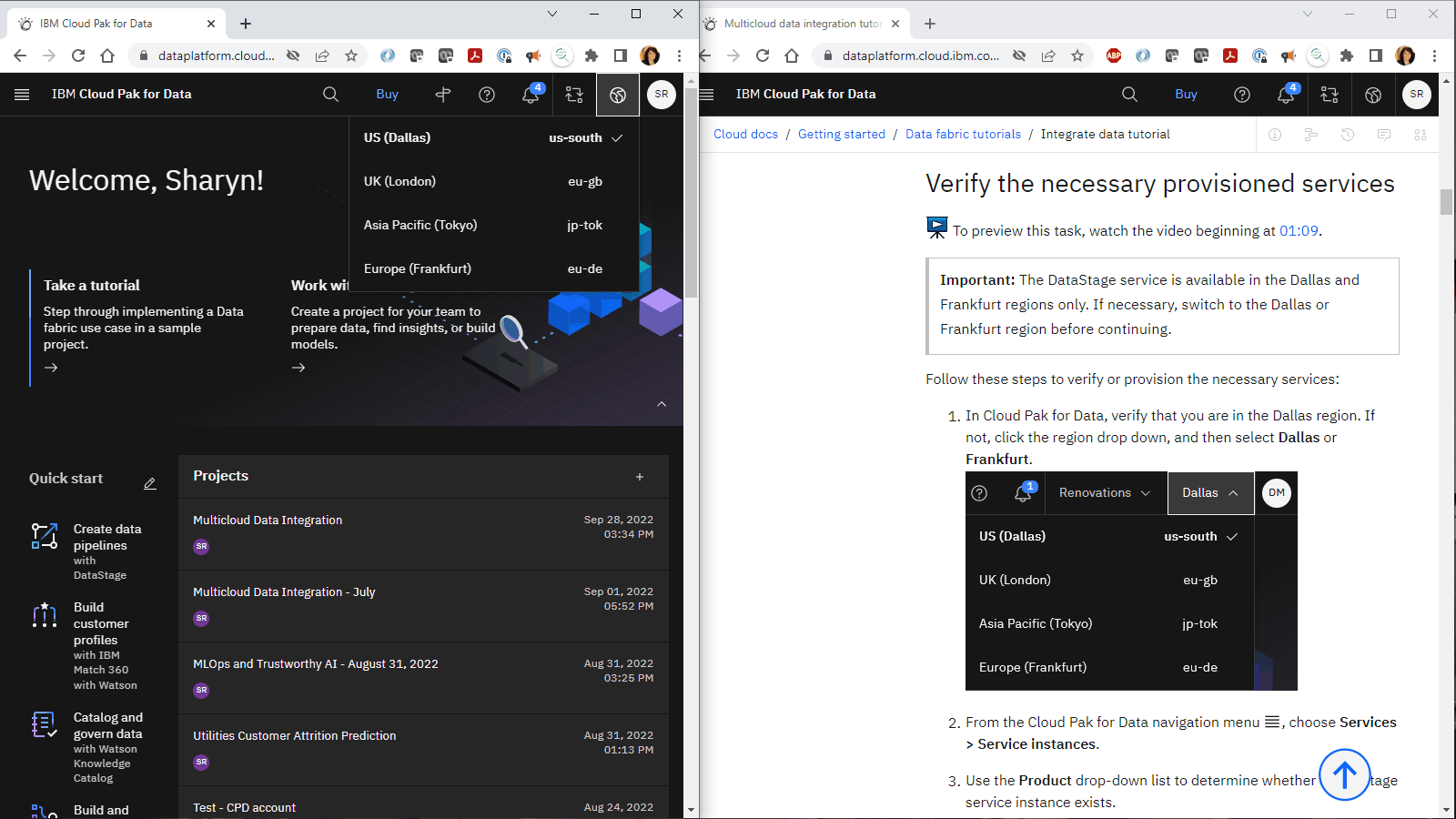
Set up your browser windows
For the optimal experience completing this tutorial, open Cloud Pak for Data in one browser window, and keep this tutorial page open in another browser window to switch easily between the two applications. Consider arranging the two browser windows side-by-side to make it easier to follow along.
Task 1: Create a project based on a sample
 To preview this task, watch the video beginning at 00:06.
You need a project to store the assets used to build the model. For example, the training data, the AutoAI experiement or Jupyter notebook, and the saved model. Follow these steps to create a project based on a sample:
-
Access the Evaluate an ML model sample project in the Resource hub.
-
Click Create project.
-
If prompted to associate the project to a Cloud Object Storage instance, select a Cloud Object Storage instance from the list.
-
Click Create.
-
Wait for the project import to complete, and then click View new project to verify that the project and assets were created successfully.
-
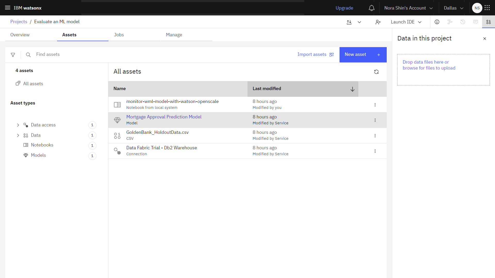
Click the Assets tab to view the assets in the sample project.
-
View the Mortgage Approval Prediction Model. This model predicts if a mortgage applicant should be approved based on several factors, such as their credit history, total debt, income, loan amount, and employment history.
-
Return to the project's Assets tab.
 Check your progress
The following image shows the sample project. You are now ready to start the tutorial.
Task 2: Deploy the model
Before you can deploy the model, you need to promote the model to a new deployment space. Deployment spaces help you to organize supporting resources such as input data and environments; deploy models or functions to generate predictions or solutions; and view or edit deployment details. The next task is to promote the evaluation data and the model to a deployment space, and then create an online deployment.
Task 2a: Download the evaluation data
 To preview this task, watch the video beginning at 00:34.
To validate that the model is working as required, you need a set of labeled data, which was held out from model training. The sample project includes the evaluation data (GoldenBank_HoldoutData.csv), which you can upload to perform the evaluation in the deployment space later. Follow these steps to download the data set:
-
Click the Overflow menu
for the GoldenBank_HoldoutData.csv data asset, and choose Download.
-
Save the data asset to your computer.
Task 2b: Promote the model to a deployment space
 To preview this task, watch the video beginning at 00:42.
Before you can deploy the model, you need to promote the model to a deployment space. Follow these steps to promote the model to a deployment space:
-
From the Assets tab, click the Overflow menu
for the Mortgage Approval Model model, and choose Promote to space.
-
Choose an existing deployment space. If you don't have a deployment space:
-
Click Create a new deployment space.
-
For the name, type:
Golden Bank Preproduction Space -
Select a storage service.
-
Select a machine learning service.
-
Select Development for the Deployment stage.
-
Click Create.
-
Close the notification when the space is ready.
-
-
Select the Go to the model in the space after promoting it option.
-
Click Promote.
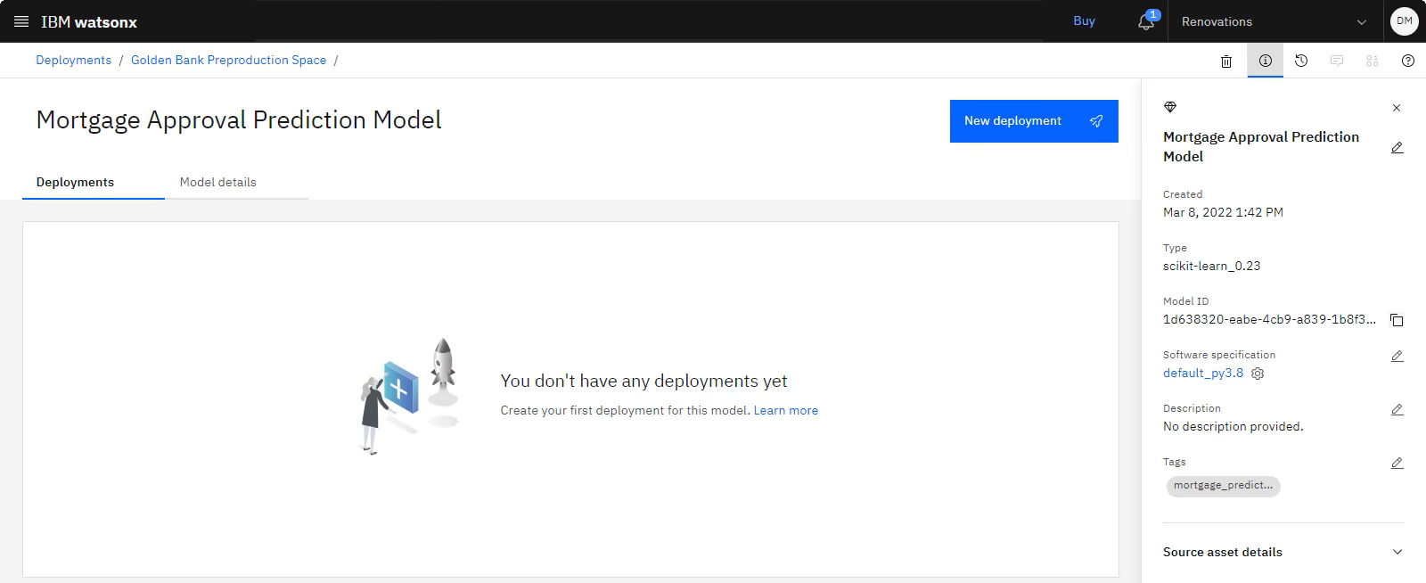
 Check your progress
The following image shows the model in the deployment space.
Task 2c: Create a model deployment
 To preview this task, watch the video beginning at 01:02.
Now that the model is in the deployment space, follow these steps to create the model deployment:
-
With the model open, click New deployment.
-
Select Online as the Deployment type.
-
For the deployment name, type:
Mortgage Approval Model Deployment -
Click Create.
-
-
When the deployment is complete, click the deployment name to view the deployment details page.
-
Review the scoring endpoint, which you can use to access this model programmatically in your applications.
 Check your progress
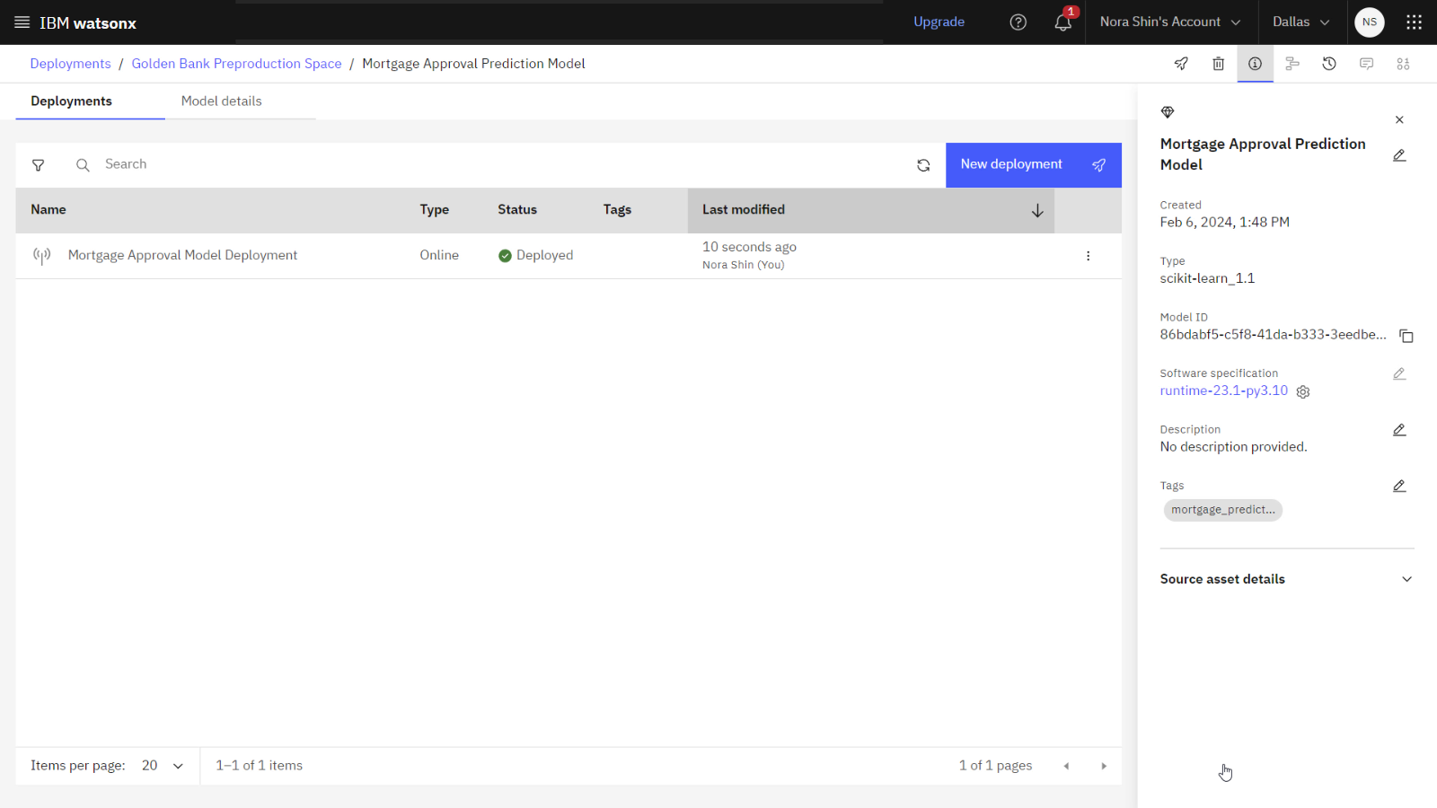
The following image shows the model deployment in the deployment space.
Task 3: Configure evaluations in a deployment space
 To preview this task, watch the video beginning at 01:19.
Follow these steps to configure evaluations in this deployment space:
Task 3a: Configure the model details
First. follow these steps to configure the model details.
- In the deployment, click the Evaluations tab.
- Click Configure OpenScale evaluation settings.
Specify model input
The training data contains numerical and categorical data that is suitable for a binary classification model.
- For Data type, select Numeric/categorical.
- For the Algorithm type, select Binary classification.
- Click View summary.
- Review the summary, and click Save and Continue.
Connect to the training data
The training data is stored in a Db2 Warehouse on Cloud instance.
- For Configuration method, select Use manual setup.
- Click Next.
- For the Training data option, select Database or cloud storage.
- Select Db2 for the location.
- Provide the connection information:
- Hostname or IP address:
db2w-ruggyab.us-south.db2w.cloud.ibm.com - SSL port:
50001 - Database:
BLUDB - Username:
CPDEMO - Password:
DataFabric@2022IBM
- Hostname or IP address:
- Click Connect.
- Select AI_MORTGAGE for the Schema.
- Select MORTGAGE_APPROVAL_TABLE for the table.
- Click Next.
Select the features and label columns
The MORTGAGE_APPROVAL column indicates whether the applicant is approved, and the feature columns contain information that contributes to the approval decision.
-
Review the following feature columns:
- GENDER
- EDUCATION
- EMPLOYMENT_STATUS
- MARITAL_STATUS
- INCOME
- APPLIEDONLINE
- RESIDENCE
- YRS_AT_CURRENT_ADDRESS
- YRS_WITH_CURRENT_EMPLOYER
- NUMBER_OF_CARDS
- CREDITCARD_DEBT
- LOANS
- LOAN_AMOUNT
- CREDIT_SCORE
- COMMERCIAL_CLIENT
- AREA_AVG_PRICE
- COMM_FRAUD_INV
- PROPERTY_VALUE
-
Search for
MORTGAGE_APPROVAL, and select the Label/Target checkbox. -
Click Next.
Specify model output details
From the model output data, you need to select the prediction column generated by the deployed model, and the probability column, which contains the model's confidence in the prediction.
- Select the appropriate checkboxes for the Prediction and Probability columns.
- Click View summary.
- Click Finish.
 Check your progress
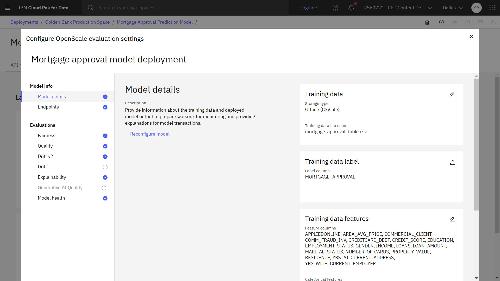
The following image shows the completed model details. Now you are ready to configure explainability.
Task 3b: Configure explainability
 To preview this task, watch the video beginning at 02:58.
Next, follow these steps to configure explainability.
Select the explanation method
Shapley Additive Explanations, or SHAP, uses all possible combinations of inputs to discover how each input moves a prediction toward or away from a mean prediction value or confidence score. Local interpretable model-agnostic explanations, or LIME, builds sparse linear models to discover the importance of each feature. SHAP is more thorough, and LIME is faster.
- Click Explainability.
- Next to Parameters, click the Edit icon
.
- Toggle on the Global explanation option.
- For the Global explanatiion method, select LIME (enhanced).
- For the Local explanatiion method, select LIME (enhanced).
- Click Next.
Configure global explanability
SHAP quantifies the influence that each feature makes on the model outcome. SHAP produces a summary plot that is suitable for global explanations, but can also generate single prediction explanations.
- Review the settings, and accept the default values in the following sections:
- Global explanation settings
- LIME settings
- Click Next.
Select the controllable features
You can specify the features you want to be controllable when running an analysis to show which features were most important in determining the model outcome.
- Review the list of controllable features.
- Click Save.
 Check your progress
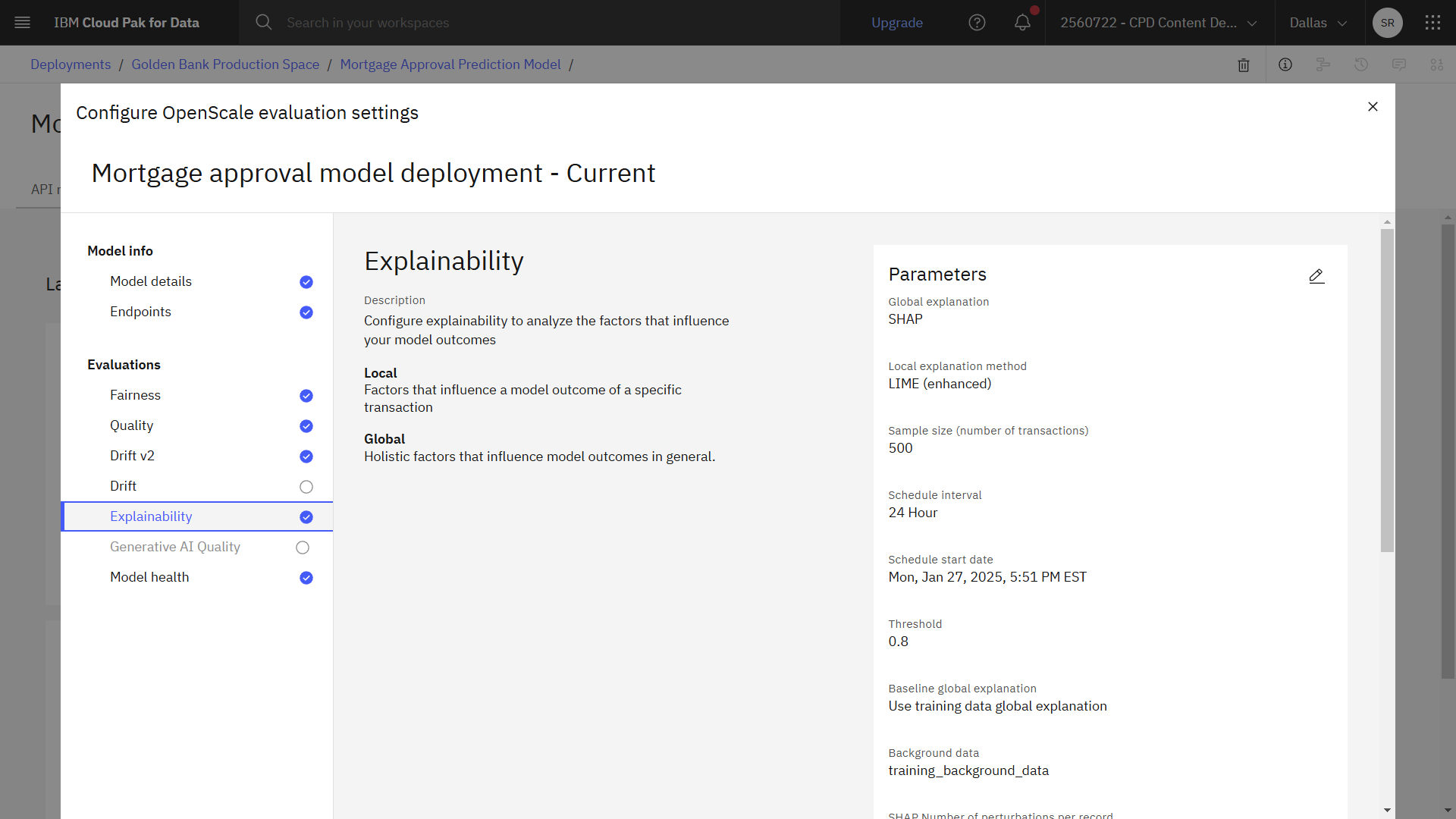
The following image shows the completed explainability configuration. Now you are ready to configure fairness.
Task 3c: Configure fairness
 To preview this task, watch the video beginning at 04:06.
Next, follow these steps to configure fairness.
Select a configuraion type
You can either configure fairness manually, or upload a configuration file generated using the supplied Jupyter notebook.
- Click Fairness.
- Next to Configuration, click the Edit icon
.
- Select Configure manually for the Configuration type.
- Click Next.
Select the favorable outcomes
For this model deployment, a favorable outcome is when an applicant is approved for a mortgage, and an unfavorable outcome is when an applicant is not approved.
- In the table, select Favorable for the 1 value, which represents that the applicant is approved for a mortgage.
- In the table, select Unfavorable for the 0 value, which represents that the applicant is not approved for a mortgage.
- Click Next.
Sample size
Adjust the sample size based on the data set that you will use to evaluate the model.
- Change Minimum sample size to
100. - Click Next.
Metrics
The Fairness monitor tracks multiple fairness metrics. The disparate impact is the ratio of the percentage of favourable outcomes for the monitored group to the percentage of favourable outcomes for the reference group.
- Review the monitored metrics generated from all data to apply to monitored features, and then review metrics generated from feedback data to apply to monitored features.
- Accept the default metrics, and click Next.
- Accept the default values for the lower and upper thresholds, and click Next.
Select the fields to monitor
You want to monitor the deployed model's tendency to provide a favorable outcome for one group over another. In this case, you want to monitor the model for gender bias.
- Select the GENDER field.
- Click Next.
- If the values are listed in the table:
- Check Female: Monitored
- Check Male: Reference.
- If the values are not listed in the table:
- In the Add custom value field, type
Female. - Click Add value.
- Select Monitored next to Male in the table.
- In the Add custom value field, type
Female. - Click Add value.
- Select Reference next to Male in the table.
- In the Add custom value field, type
- Click Next.
- Accept the default threshold for the monitored group, and click Save.
 Check your progress
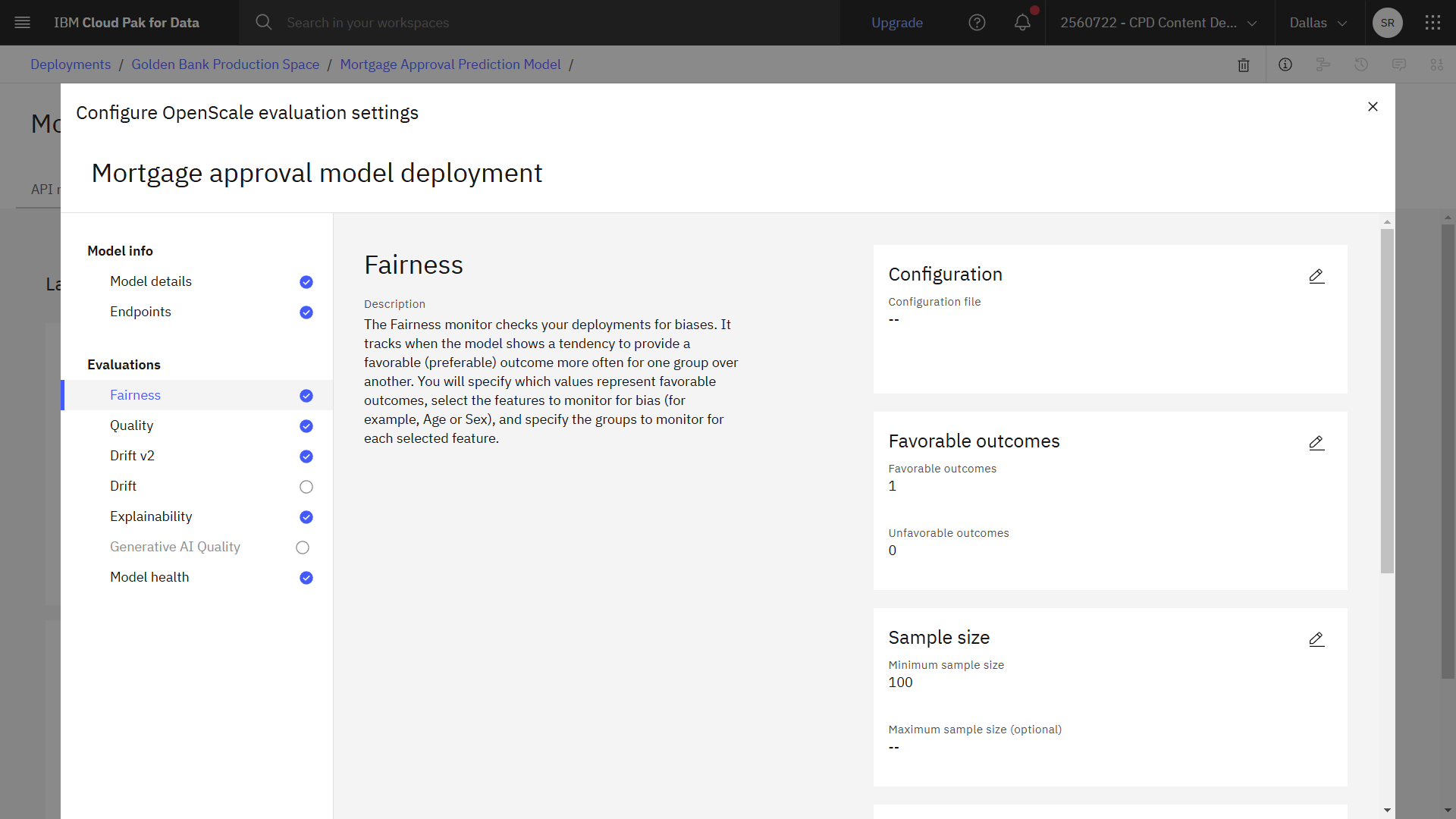
The following image shows the completed fairness configuration. Now you are ready to configure quality.
Task 3d: Configure quality
 To preview this task, watch the video beginning at 05:17.
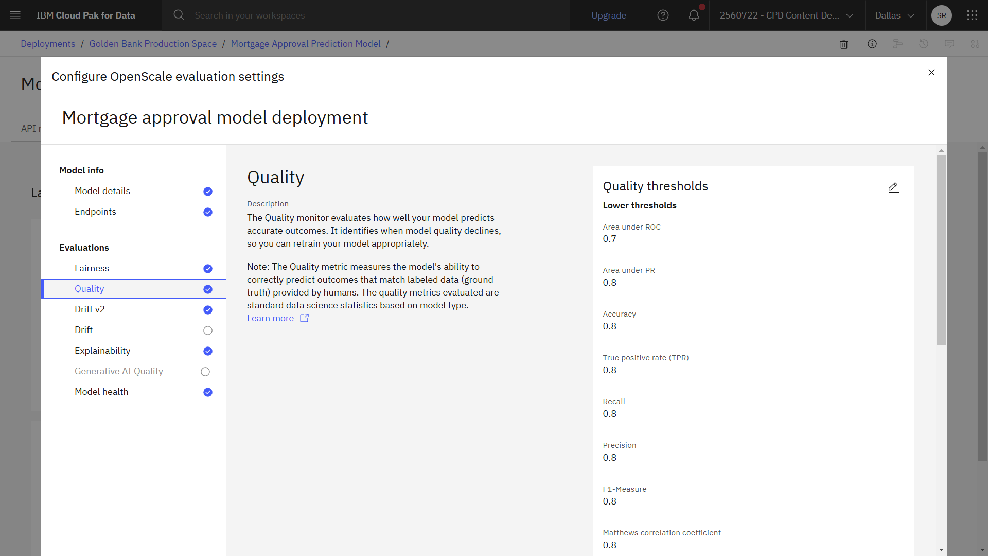
Next, follow these steps to configure quality. The Quality monitor evaluates how well your model predicts accurate outcomes.
- Click Quality.
- Next to Quality thresholds, click the Edit icon
.
- Change the value for Area under ROC to
0.7. - Click Next.
- Change the Minimum samples size to
100. - Click Save.
 Check your progress
The following image shows the completed quality configuration. Now you are ready to configure drift.
Task 3e: Configure drift
 To preview this task, watch the video beginning at 05:42.
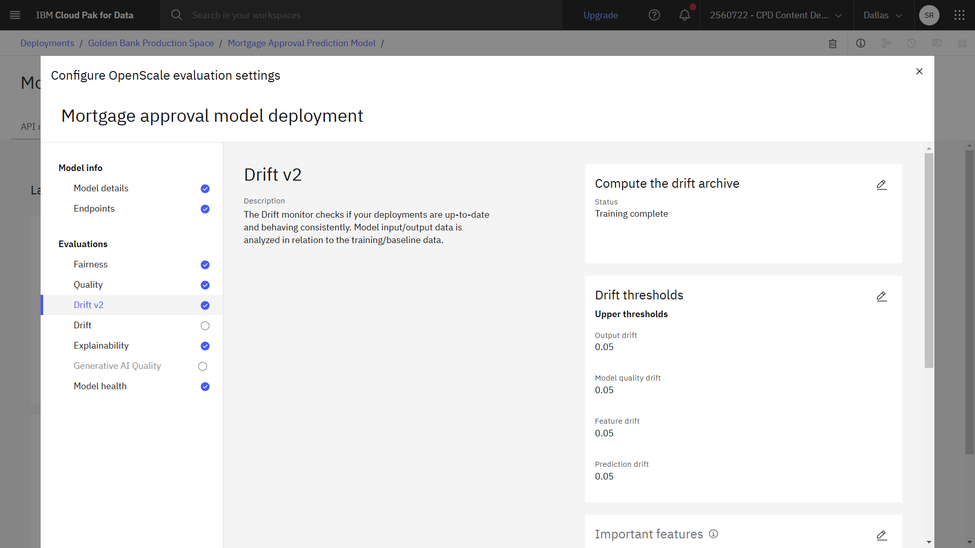
Lastly, follow these steps to configure drift. The Drift monitor checks if your deployments are up-to-date and behaving consistently.
- Click Drift v2.
- Next to Compute the drift archive, click the Edit icon
.
- For the Compute option, select Compute in Watson OpenScale. This option tells Watson OpenScale to perform an analysis of your training data to determine the data distributions of the features.
- Click Next.
- Accept the default values for upper thresholds, and click Next.
- For the Important features, select all columns, and click Next.
- For Most important features, select the following columns, and click Next.
- CREDITCARD_DEBT
- INCOME
- LOANS
- LOAN_AMOUNT
- PROPERTY_VALUE
- Accept the default values for sample size, and click Save.
- Click the X to close the window and wait for Watson OpenScale to fetch the monitors.
 Check your progress
The following image shows the completed configuration in the deployment space. Now you are ready to monitor the model deployment.
Task 4: Evaluate the model
 To preview this task, watch the video beginning at 06:22.
Follow these steps to use holdout data to evaluate the model:
-
From the Actions menu, select Evaluate now.
-
From the list of import options, select from CSV file.
-
Drag the Golden Bank_HoldoutData.csv data file you downloaded from the project into the side panel.
-
Click Upload and evaluate and wait for the evaluation to complete.
-
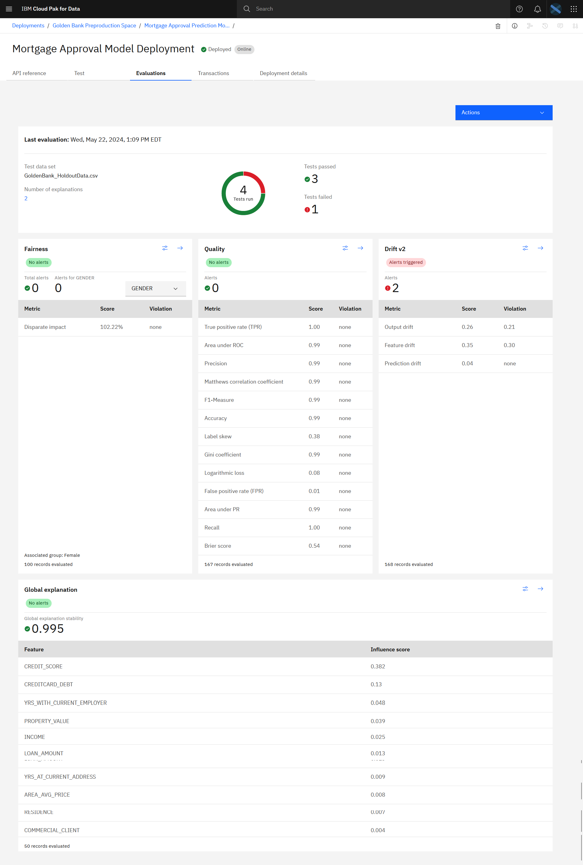
When the evaluation completes, you will see the number of tests run, tests passed, and tests failed. Scroll to see the results for Fairness, Quality, Drift, and Global explanation.
 Check your progress
The following image shows the result of the evaluation for the deployed model. Now that you evaluated the model, you are ready to observe the model quality.
Task 5: Observe the model monitors for quality
 To preview this task, watch the video beginning at 06:36.
The Watson OpenScale quality monitor generates a set of metrics to evaluate the quality of your model. You can use these quality metrics to determine how well your model predicts outcomes. When the evaluation that uses the holdout data completes, follow these steps to observe the model quality or accuracy:
-
In the Quality section, click the Configure icon
 . Here you can see that the quality threshold
that is configured for this monitor is 70% and that the measurement of quality being used is area under the ROC curve.
 -
Click the X to close the window and return to the model evalution screen.
-
In the Quality section, click the Details icon
 to see the model quality detailed results.
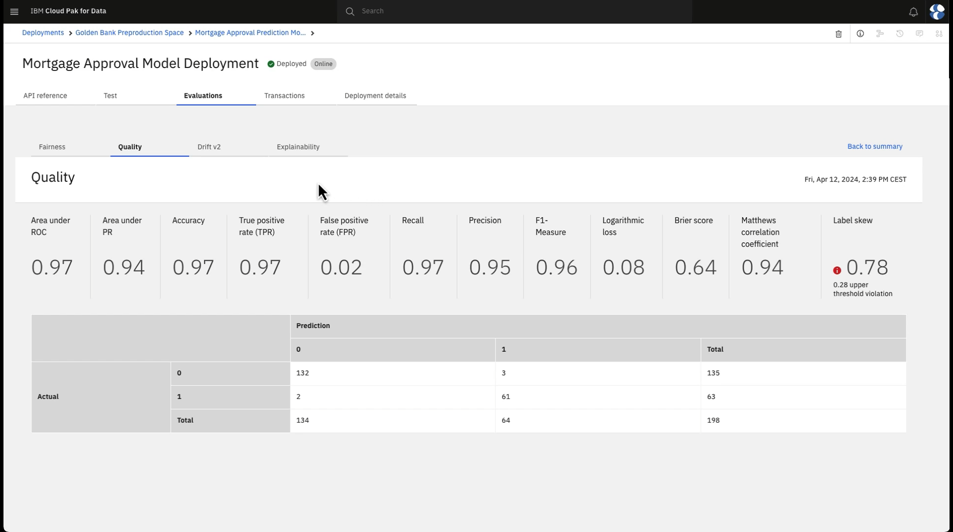
Here you see a number of quality metric calculations and a confusion matrix showing correct model decisions along with false positives and false negatives. The calculated area under the ROC curve is 0.9 or higher, which exceeds the
0.7 threshold, so the model is meeting its quality requirement.
 -
Click Back to summary to return to the model details screen.
 Check your progress
The following image shows the quality details in Watson OpenScale. Now that you observed the model quality, you can observe the model fairness.
Task 6: Observe the model monitors for fairness
 To preview this task, watch the video beginning at 07:20.
The Watson OpenScale fairness monitor generates a set of metrics to evaluate the fairness of your model. You can use the fairness metrics to determine if your model produces biased outcomes. Follow these steps to observe the model fairness:
-
In the Fairness section, click the Configure icon
 . Here you see that the model is being
reviewed to ensure that applicants are being treated fairly regardless of their gender. Women are identified as the monitored group for whom fairness is being measured and the threshold for fairness is to be at least 80%. The fairness
monitor uses the disparate impact method to determine fairness. Disparate impact compares the percentage of favorable outcomes for a monitored group to the percentage of favorable outcomes for a reference group.
 -
Click the X to close the window and return to the model evalution screen.
-
In the Fairness section, click the Details icon
 to see the model fairness detailed results.
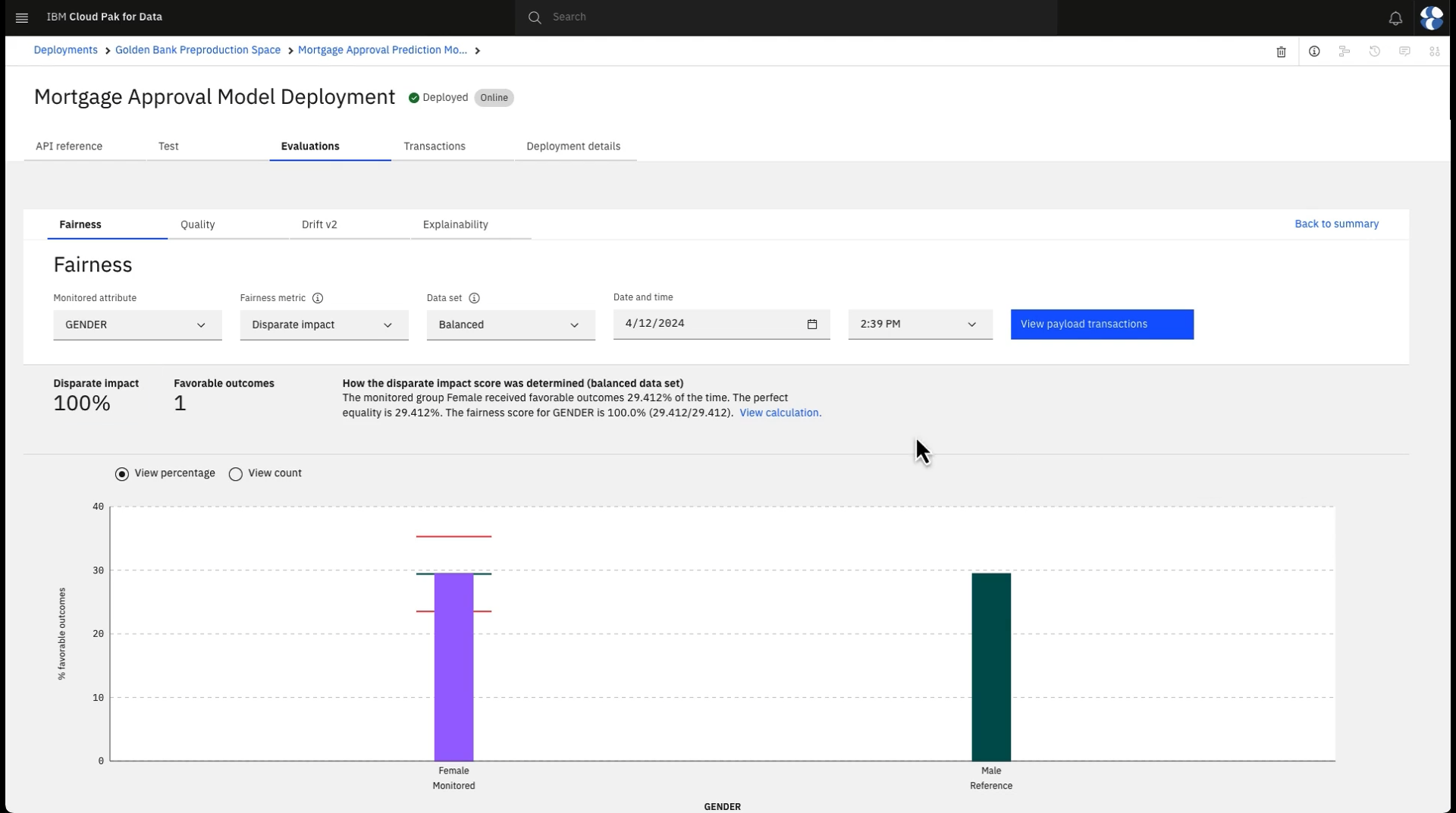
Here you see the percentage of male and female applicants who are being automatically approved, along with a fairness score of over 100%, so the model performance far exceeds the 80% fairness threshold required.
 -
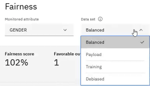
Note the identified data sets. To ensure that the fairness metrics are most accurate, Watson OpenScale uses perturbation to determine the results where only the protected attributes and related model inputs are changed while other features remain the same. The perturbation changes the values of the feature from the reference group to the monitored group, or vice-versa. These additional guardrails are used to calculate fairness when the "balanced" data set is used, but you can also view the fairness results using only payload or model training data. Since the model is behaving fairly, you don't need to go into additional detail for this metric.
-
Click Back to summary to return to the model details screen.
 Check your progress
The following image shows the fairness details in Watson OpenScale. Now that you observed the model fairness, you can observe the model explainability.
Task 7: Observe the model monitors for drift
 To preview this task, watch the video beginning at 08:25.
The Watson OpenScale drift monitor measures changes in your data over time to ensure consistent outcomes for your model. Use drift evaluations to identify changes in your model output, the accuracy of your predictions, and the distribution of your input data. Follow these steps to observe the model drift:
-
In the Drift section, click the Configure icon
 . Here you see the drift thresholds. Output
drift measures the change in the model confidence distribution. Model quality drift measures the drop in accuracy by comparing the estimated runtime accuracy to the training accuracy. Feature drift measures the change in value distribution
for important features. The configuration also shows the number of selected features and the most important features.
 -
Click the X to close the window and return to the model evalution screen.
-
In the Drift section, click the Details icon
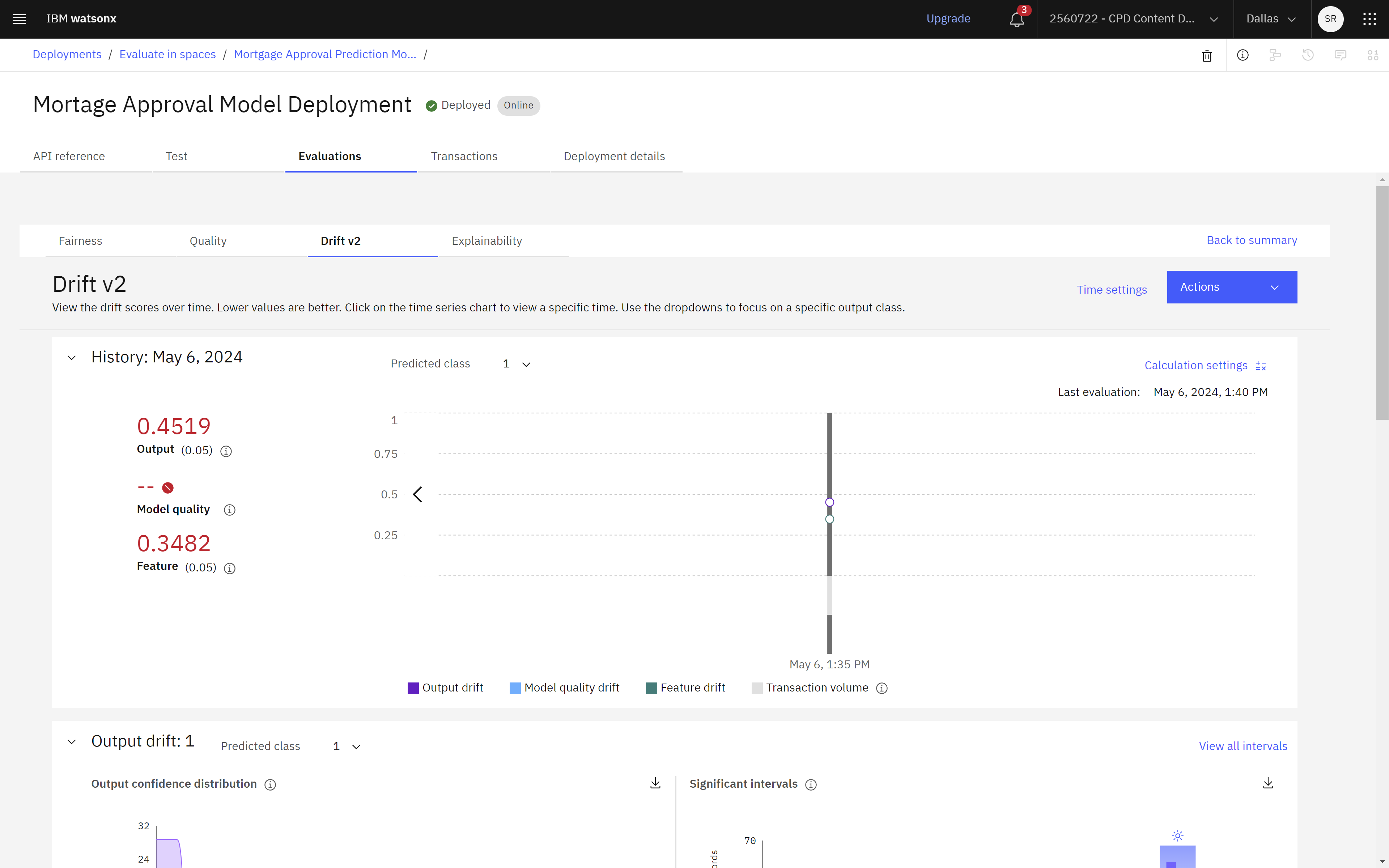
 to see the model drift detailed results. You
can view the history of how each metric score changes over time with a time series chart. Lower values are better, so in this case, the results are above the upper thresholds that are set in the configuration. Then view details about
how the scores output and feature drifts are calculated. You can also view details about each feature to understand how they contribute to the scores that Watson OpenScale generates.
 -
Click Back to summary to return to the model details screen.
 Check your progress
The following image shows the drift details in Watson OpenScale. Now that you observed the model drift, you can observe the model explainability.
Task 8: Observe the model monitors for explainability
 To preview this task, watch the video beginning at 09:10.
It is also important to understand how the model came to its decision. This understanding is required both to explain decisions to people involved in the loan approval and to ensure model owners that the decisions are valid. To understand these decisions, follow these steps to observe the model explainability:
-
Click the Transactions tab.
-
On the graph, select a timeframe to see a list of transactions during that period.
-
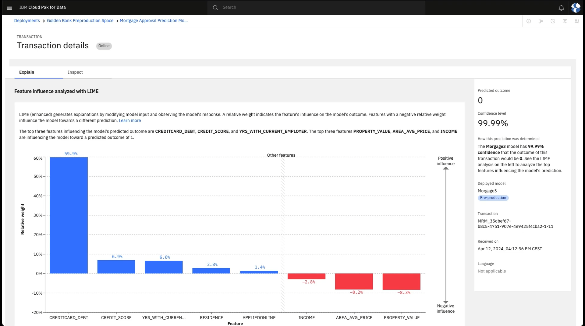
For any transaction, click Explain under the Actions column. Here you see the detailed explanation of this decision. You will see the most important inputs to the model along with how important each was to the end result. Blue bars represent inputs that tended to support the model's decision while red bars show inputs that might have led to another decision. For example, an applicant might have enough income to otherwise be approved but their poor credit history and high debt together lead the model to reject the application. Review this explanation to become satisfied about the basis for the model decision.
-
Optional: If you want to delve further into how the model made its decision, click the Inspect tab. Use the Inspect feature to analyze the decision to find areas of sensitivity where a small changes to a few inputs would result in a different decision, and you can test the sensitivity yourself by overriding some of the actual inputs with alternatives to see whether these would impact the result. Click Run analysis to have Watson OpenScale reveal the minimum changes required to deliver a different outcome. Select Analyze controllable features only to limit changes to the controllable features only.
 Check your progress
The following image shows the explainability of a transaction in Watson OpenScale. You have determined that the model is accurate and treating all applicants fairly. Now, you can advance the model to the next phase in its lifecycle.
Next steps
Try these additional tutorials:
Additional resources
Parent topic: Quick start tutorials